This post provides you an easy to follow tutorial on how to “train a base neural net” on a dataset and use that pre-trained network to “transfer learn” on a different dataset using MXNet/Gluon framework.

Table of contents:

1. Data used
   1. IMDB
   2. Hotel
2. Imports
3. Step 1. Sklearn Data Transformations
4. Step 2. MXNet Dataset and Dataloaders
5. Step 3. MXNet Custom Networks
6. Step 4. Training Base Model
7. Step 5. Extracting Embeddings from the Network
8. Step 6. Transfer Learning on a Different Dataset
   1. Weights as it is:
   2. Weights as feature extractor:
   3. Weights as initializations:
   4. Save and load the model
   5. Train the network on new dataset
9. Conclusion
10. End

Transfer learning (TL) is a research problem in machine learning (ML) that focuses on storing knowledge gained while solving one problem and applying it to a different but related problem. For example, knowledge gained while learning to recognize cars could apply when trying to recognize trucks - wiki definition.

This post provides you an easy to follow tutorial on how to “train a base neural net” on a dataset and use that pre-trained network to “transfer learn” on a different dataset using MXNet/Gluon framework. The high level steps in this tutorial are very similar for any kind of transfer learning problem - tabular, time series, language or computer vision. The major differences when working with different problems are “network architecture” and “transformations and pre-processesing steps”. My goal is to provide a skeletal using text data (movie and hotel reviews) as an example, that you can adapt for different tasks. I have primarily used MXNet, Catboost and Sklearn libraries for this post. Here is the link to the jupyter notebook in case you directly want to jump to the code and skip reading the explainations.

I haven’t covered any theory about what is transfer learning, why and where is it useful. To learn more on the theory part, I recommend this post by Sebastian Ruder - Transfer Learning - Machine Learning’s Next Frontier. Ruder has done his PhD in this topic. So his work is really detailed. Here is the link to his thesis for deep divers.

The post and notebook combined give you tutorial to the the following things. These topics are also independent tutorials and can be ripped off to use for other problems as well.

1. How to write sklearn transformers?
2. How to create a custom neural net architecture on MXNet?
3. How to train a network on MXNet?
4. How to extract and visualize embeddings from any layer of the trained model using t-SNE?
5. How to save and load a trained MXNet network
6. How to freeze/unfreeze any layer in MXNet?
7. How to relearn network parameters using a new dataset?

So let’s dive right in!

Data used

I have used IMDB movie reviews dataset to train the base network and transfered the learning done from this base network to Hotel reviews dataset. In general, transfer learning is more useful on smaller or unlabelled data whereas base networks are trained on larger datasets. (Shared links might not be the original source of these datasets. These are just the links I used for my analysis).

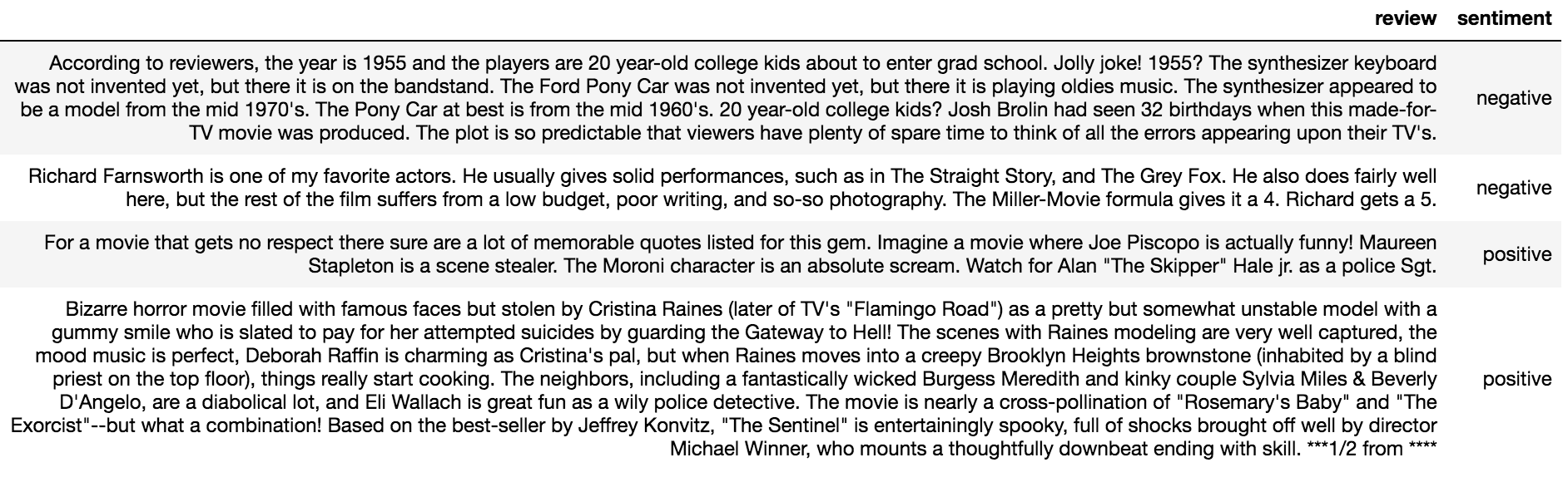
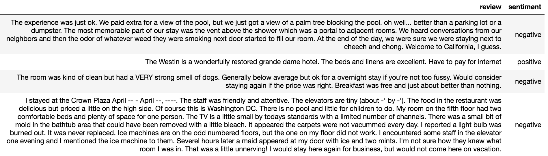
Both of these datasets contain reviews and a label about whether the review has a positive or a negative sentiment. (movie reviews from IMDB and hotel reviews from Hotel dataset). Therefore, both of these datasets are similar but from very different domains which makes it a good use case for transfer learning. Let’s see how well we can transfer knowledge from movie reviews to hotel reviews.

Examples from both datasets.

IMDB

Total of 25k reviews. 12.5k positive, 12.5k negative

Hotel

Total of 38.9k reviews. 26.5k positive, 12.4k negative

Imports

Here, putting a code block of all the libraries that are used for this tutorial.

# basic utils for data preparation, plotting
import os, sys, time, math, ast, re, string, random
from collections import defaultdict
import datetime
import joblib, boto3
import pandas as pd
import numpy as np
import matplotlib.pyplot as plt
import seaborn as sns
import boto3
import gzip
import tarfile
from io import StringIO

# mxnet/gluon/gluonnlp 
import mxnet as mx
from mxnet import gluon, autograd
import mxnet.ndarray as nd
import gluonnlp as nlp

# sklearn ML stuff
from sklearn.model_selection import train_test_split
from sklearn.metrics import roc_auc_score
from sklearn.feature_extraction.text import TfidfVectorizer
from sklearn.linear_model import LogisticRegression
from sklearn.preprocessing import normalize

# For creating sklearn transformers
from sklearn.pipeline import Pipeline
from sklearn.impute import SimpleImputer
from sklearn.compose import ColumnTransformer
from sklearn.base import BaseEstimator, TransformerMixin

Step 1. Sklearn Data Transformations

The raw data is hardly clean enough to be used directly. There is always some form of data cleaning and pre-processing required to be done on any data before training an ML model. The type and amount of cleaning/pre-processing varies with the data and the choice of ML algorithm.

This particular task requires minimal data transformations as mentioned below.

1. Replace missing reviews with a token - “null”.
2. Lower case all the text. (Language learning tasks can actually perform better without lower casing. For e.g., “AWESOME” vs “awesome” can show different levels of positive sentiments.)
3. Tokenize the text. Tokenization example: [“the room was kind of clean”] → [“the”, “room”, “was”, “kind”, “of”, “clean”].
4. Assign each token (e.g. “the”, “room”, “was”) an integer index. Our neural net will only takes in numbers, not words and we pass in sequence of numbers to learn the language structure.

If you have used Sklearn library before, I am sure you would be familiar with .fit() and .transform() methods. You generally fit an algorithm on training data using .fit() method and apply the trained model on the test data using .transform() or .predict(). You can adapt any transformer or a custom algorithm into this class structure. Just create a custom data transformation pipeline using the same Sklearn interface. It helps you to package your code so that it’s easy to use for both experiements and production, and reproducible for different datasets. Here is official page to sklearn pipelines. Below is how a data transformation pipeline looks like

# Transformers present in Pipeline work in series. 1->2->3->4
transformer_pipe = Pipeline(steps=[
("null_impute", NullImputer(strategy="constant", fill_value="null")),
("lower_case", LowerCaser()),
("tokenize", Tokenize(f"([{string.punctuation}])")),
("token2index", Tok2Idx())
])

X_train_transformed = transformer_pipe.fit_transform(X_train) # fit and transform on train data
X_valid_transformed = transformer_pipe.transform(X_valid)
X_test_transformed = transformer_pipe.transform(X_test)

# saving transformer to a file for later use 
# we need to apply same transformation when we need to ...
# evaluate models on new datasets (batch transform or real time inference)
joblib.dump(transformer_pipe, "filepath")

# loading the saved transformer
transformer_pipe = joblib.load("filepath")

# you can also build a column transformer that applies different pipelines to different 
# set of features and then combine all of the transfromed features together
# e.g.
from sklearn.compose import ColumnTransformer
column_transformer = ColumnTransformer(transformers=[
    ("pipeline1", transformer_pipe1, ["list-of-features1"]),
    ("pipeline2", transformer_pipe2, ["list-of-features2"])
])

Breaking down: The pipeline above comprises of 4 custom transformers defined using the Sklearn base estimator class. By definition, all steps in a pipeline object run in sequence. i.e. it first fills missing values, then converts strings to lower case, then tokenizes using string punctuations and at the end converts tokens into interger indexes. The input to output map looks like below.

# After first fitting on the IMDB training data
transformer_pipe.transform(pd.Series(["This is just an example.",
                                      "This is another example"]))
                                

Output:
0    [1192, 40267, 3049, 50090, 51984, 62589]
1    [1192, 40267, 53296, 51984]

Let’s look at how each of these transformers are defined. You basically inherit functionalities from Sklearn’s BaseEstimator and TransformerMixin, and overwrite fit() and transform() methods as per your requirements.

class Tokenize(BaseEstimator, TransformerMixin):
    """
    Takes in pandas series and applies tokenization on each row based on given split pattern. 
    """
    def __init__(self, split_pat=f"([{string.punctuation}])"):
        self.split_pat = split_pat  # re pattern used to split string to tokens. default splits over any string punctuation
    
    def tokenize(self, s):
        """ Tokenize string """
        re_tok = re.compile(self.split_pat)
        return re_tok.sub(r' \1 ', s).split()  # substitute all delimiters specified in pattern with space and then splits over space
    
    def fit(self, X, y=None):  # no need to learn anything from training data for tokenization. so returning self
        return self

    def transform(self, X, y=None):
        return X.apply(self.tokenize)
    
    
class Tok2Idx(BaseEstimator, TransformerMixin):
    """
    Creates integer index from tokenizes columns. 
    Creates a dictionary of all unique tokens and corresponding integer index
    Transform maps any token unseen in the training data to <unk> token 
    Need pandas series as input. 
    """
            
    def map_tok_idx(self, char):
        try:
            return self.tok2idx[char]
        except KeyError:
            return self.tok2idx["<unk>"]

    def fit(self, X, y=None):
        """ To be called for training data. Creates a token to integer map """
        self.uniq_set = list(set([y for x in list(X.values) for y in x]))
        self.uniq_set.append("<unk>")
        self.tok2idx = {j:i for i,j in enumerate(self.uniq_set)}
        self.idx2tok = {i:j for i,j in enumerate(self.uniq_set)}
        return self

    def transform(self, X, y=None):
        return X.map(lambda x: [self.map_tok_idx(c) for c in x])
    
    
class LowerCaser(BaseEstimator, TransformerMixin):
    """
    Lower case all string values. 
    Need pandas series as input. 
    No fitting is required for this one.
    """
    def transform(self, X, y=None):
        return X.str.lower()
    
    
class NullImputer(SimpleImputer):
    """
    SimpleImputer works with 2D array. For the purpose of this analysis, we are working with pd Series. 
    Modifying it a bit
    """
    def __init__(self, missing_values=np.nan, strategy='mean', fill_value=None, **kw):
        super(NullImputer, self).__init__(
            missing_values=missing_values,
            strategy=strategy,
            fill_value=fill_value
        )

    def fit(self, X, y=None):
        super(NullImputer, self).fit(pd.DataFrame(X), y)
        return self

    def transform(self X):
        result = super(NullImputer, self).transform(pd.DataFrame(X))
        return pd.DataFrame(result)[0]  # converting 2D array back to series

Step 2. MXNet Dataset and Dataloaders

After these basic transformations, the next step is to prepare the dataset and feed into the neural net in small batches. The neural net parameters are trained using back propagation and it’s better to quickly update the parameters by using small batches of data than looking at all of the training data for each update (Andrew Ng on Batch vs. mini batch gradient descent). To make this preparation of batches and loading of data easy, DL frameworks provide Dataset and Dataloader classes that can be customized for problem at hand.

Dataset class provides a nice way to load different types of data that can be indexed and sliced. For the problem under discussion, we want our dataset to load sequence of integers obtained using the data transformation and sentiment label for each review. Gluon has a multiple dataset wrappers over abstract dataset class. You can either create your own dataset by inheriting from dataset class or use one of the wrappers. In this case, we use SimpleDataset wrapper which works for data that is in the form of array and list.

max_seq_len = 555 # 90% of reviews have word/token length smaller than this

# Clip if the review length becomes larger than max_seq_len
train_dataset = gluon.data.SimpleDataset(list(zip(transformed_reviews,
                                            labels))).\
transform(lambda review, label: (nlp.data.ClipSequence(max_seq_len)(review), label))

# indexing on ith row of train data will give
# sequence of integers which are output of data transformation (X) 
# and a sentiment label (y).  
train_dataset[0] == [[1192, 40267, 3049, 50090, 51984, 62589],0]
len(train_dataset) == 16000

For training, we need to create mini batches of data by shuffling and slicing the dataset object. Rather than doing this process manually in loops, we use inbuilt functionality of Dataloaders. Dataloader takes in a dataset object and other parameters like whether to shuffle or not, how to shuffle, required batch size, how to pad sequences, bucketing similar size arrays together, number of concurrent workers to use etc. It then creates a generator that returns batches of data for training.

def get_dataloader(dataset,
                   dataset_type="train",  # valid/test
                   batch_size=256,
                   bucket_num=5,
                   shuffle=True,  # true for training
                   num_workers=1):
    
    # Batchify function appends the length of each sequence to feed as addtional input 
    combined_batchify_fn = nlp.data.batchify.Tuple(
        nlp.data.batchify.Pad(axis=0, ret_length=True),
        nlp.data.batchify.Stack(dtype='float32'))  # stack input samples
  
    if dataset_type == "train":
        data_lengths = dataset.transform(
            lambda review, label: float(len(review)), lazy=False)
    
        # We need to shuffle for training data.
        # It's more efficient to shuffle training data such that sequences with similar length come together
        # This is achieved using FixedBucketSampler
        batch_sampler = nlp.data.sampler.FixedBucketSampler(
            data_lengths,
            batch_size=batch_size,
            num_buckets=bucket_num,
            shuffle=shuffle)

        dataloader = gluon.data.DataLoader(
            dataset=dataset,
            batch_sampler=batch_sampler,
            batchify_fn=combined_batchify_fn,
            num_workers=num_workers,
        )
    # We don't need to shuffle for valid and test datasets
    elif dataset_type in ["valid", "test"]:
        batch_sampler = None
        dataloader = gluon.data.DataLoader(
            dataset=dataset,
            shuffle=shuffle,
            batch_size=batch_size,
            batchify_fn=combined_batchify_fn,
            num_workers=num_workers)
    else:
        raise Exception("Pass dataset type from train, dev, valid or test")

    return dataloader
    
# Example of creating dataloader
train_dataloader = get_dataloader(train_dataset,
                                  batch_size=64,
                                  bucket_num=5, # number of different buckets based on length
                                  shuffle=True,
                                  num_workers=0,
                                  dataset_type="train"

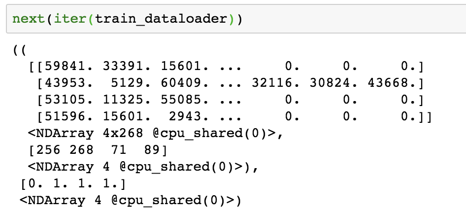
Sample output of a dataloader that uses batch size of 4 can look like following. The first part has index of integers for each token in review. The second and third parts have length and sentiment of each review respectively. Note that the rows in the first part that have shorter review length than the longest review in this batch are padded with 0.

Step 3. MXNet Custom Networks

You can use different types of network architectures as long as you can define a loss function based on the network outputs that you would like to minimize. MXNet provides large number of basic building blocks and a framework (gluon.nn) that you can use to combine various network layers and define a custom network graph.

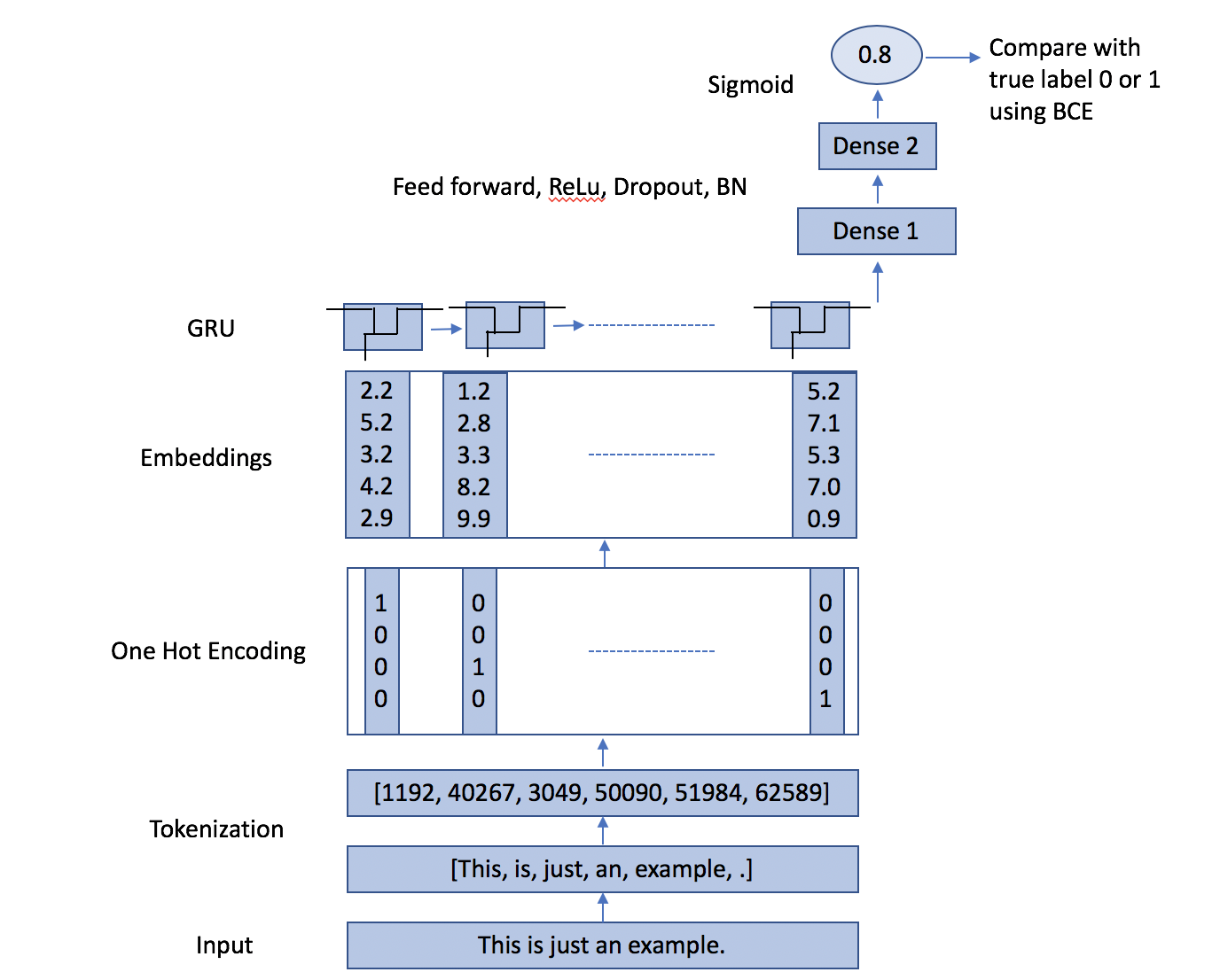
For instance, the network used in this tutorial first learns high dimentional embeddings for each token using embedding layer (a token is a word in this case). In simple words, it learns a vector for each word. The embedding vectors are then passed to a GRU layer which learns the language structure. (for theory, Illustrated Guide to LSTM’s and GRU’s: A step by step explanation). In simple words, it learns how english is written in reviews. The last output of GRU sequence is then passed to a series of linear layers with non linear activations and dropouts. The final layer returns only one number (a fraction between 0 and 1) which is used to compute the binary cross entropy (BCE) loss function. This overall network is learning which words are associated with bad sentiment vs. which words are associated with good sentiment, together with learning the language structure. I will talk more about word represenations in the next section.

class CustomSeqNet(gluon.nn.HybridBlock):
    """
    Custom defined network for sequence data that is used to predict a binary label.   
    
    """
    def __init__(self, input_output_embed_map, dense_sizes=[100], dropouts=[0.2], activation="relu"):
        """
        input_output_embed_map: {"token_embed": (max_tok_idx, tok_embed_dim), "hidden_embed": (,hidden_embed_dim))}
        """
        self.dense_sizes = dense_sizes  # list of output dimension of dense layers
        self.dropouts = dropouts  # list of dropout for each dense layer

        super(CustomSeqNet, self).__init__(prefix='CustomSeqNet_')

        with self.name_scope():  # name space object to manage parameter names
            # 1. Embedding layer
            self.embed = gluon.nn.Embedding(
                input_dim=input_output_embed_map["token_embed"][0],
                output_dim=input_output_embed_map["token_embed"][1],
                prefix='token_embed_'
            )  # output = (bs, sequence_len, input_size) = (N,T,C)
            
            # 2. GRU layer
            self.rnn = gluon.rnn.GRU(
                hidden_size=input_output_embed_map["hidden_embed"][1],
                bidirectional=True, 
                layout='NTC', # batch size, sequence length and feature dimensions respectively
                prefix='review_gru_'
            ) 

            # 3. Dense layers
            # need to specify in_units in Dense for some initialization issues
            for i, sz in enumerate(self.dense_sizes):
                setattr(self, "dense_{}".format(i), gluon.nn.Dense(sz))
                setattr(self, "bn_dense_{}".format(
                    i), gluon.nn.BatchNorm(axis=1))
                setattr(self, "activation_dense_{}".format(
                    i), gluon.nn.Activation(activation))
                setattr(self, "drop_dense_{}".format(i),
                        gluon.nn.Dropout(self.dropouts[i]))
            # 4. Output layer
            self.output = gluon.nn.Dense(1, prefix="output_")

    def hybrid_forward(self, F, review, review_len):
        embed = self.embed(review) # 1
        rnn_all = self.rnn(embed) # 2
        # Extract last output in sequence
        rnn_last = F.SequenceLast(rnn_all, sequence_length=F.cast(
            review_len, 'float32'), use_sequence_length=True)
            
        for i, sz in enumerate(self.dense_sizes): # 3
            net = getattr(self, "dense_{}".format(i))(net)  # MLP
            net = getattr(self, "bn_dense_{}".format(i))(net)  # BN
            net = getattr(self, "activation_dense_{}".format(i))(net)  # relu
            net = getattr(self, "drop_dense_{}".format(i))(net)  # dropouts
        net = self.output(net) # 4
        return net

Input arguments:

• input_output_embed_map: Dictionary with two keys. Key 1. token_embed is tuple of number of words in vocabulary and required dimension of word embedding Key 2. hidden_embed has required dimension of hidden layer in GRU
• dense_sizes: List of required output dimension from each dense layer. Network will have as many dense layers as elements of this list. Default: Single dense layer output of dim 100
• dropouts: List of required dropout in each dense layer. Default: Single dense layer output of dropout 0.2
• activation: String. Activation function. Default: “relu”.

Block is the baseclass for all neural network layers. The first line of code above CustomSeqNet(gluon.nn.HybridBlock) uses HybridBlock instead of Block to define the model. It’s similar to Block but provides an option for symbolic programming that allows fast computations. Once we call hybridize() on network, it creates a cached symbolic graph representing the forward computation. It uses that cached graph to do computation rather than calling hybrid_forward each time. This is one of the USPs of MXNet over other DL frameworks. It gives all of the benefits of imperative programming (PyTorch, Chainer) but still exploits, whenever possible, the speed and memory efficiency of symbolic programming (Theano, Tensorflow). Just call network.hybridize() and your network gets compiled to run faster.

The _init_ takes in arguments like dropouts in dense layers, size of hidden layers in GRU, size of embedding layer etc. The hybrid_forward defines the same computation graph as shown in the network architecture diagram above. 1. Embedding → 2. GRU → Last hidden layer from GRU → 3. Sequence of dense layers → 4. Final layer that gives one number as output.

Code chunk to create the network object using CustomSeqNet class.

# Preparation of network arguments
ctx = [mx.gpu(0)]  # use a GPU
tt = transformer_pipe.named_steps['token2index'] # to get token to integer map
max_idx = max(tt.tok2idx.values())+1  # size of vocabulary of all tokens in training data
tok_embed_dim = 64 # embedding size of each token
review_embed_dim = 50  # embedding size of hidden state in GRU

input_output_embed_map = {"token_embed": (max_idx, tok_embed_dim),
                         "hidden_embed": (None, review_embed_dim)}
                         
dropouts = [0.2, 0.2, 0.2]
dense_sizes=[100, 100, 10]
activation="relu"

# Network object
net1 = CustomSeqNet(input_output_embed_map, dense_sizes, dropouts, activation)

Step 4. Training Base Model

This part tells the network what it needs to do to learn the parameters based on the given data. Steps are as follows.

1. Initialize the network weights. In this case, using Xavier initializations (paper link).
2. Define which optimizer you want to use (Adam, SGD, AdaGrad etc.), your learning rate or learning rate scheduler, amount of regularization using weight decay with gluon.Trainer
3. What’s your loss function. In this case gluon.loss.SigmoidBCELoss() for binary cross entrpy loss. MXNet has many common loss functions pre-defined but you can also define a custom loss function.
4. For each mini batch
   1. Make prediction from the network using current parameters
   2. Calcualate and print loss values on training and validation sets
   3. Using chain rule on computation graph, calculate gradients for each parameter
   4. Using gradients [from step 4(iii)], perform a single step of gradient update with optimizer defined in step 2.
5. Perform step 4 multiple times upto point when you observe that validation loss is not reducing anymore or starts to increase.

The code performing steps as defined above. Note: Go to the notebook for util function evaluate_network function which gives loss value, auc and prediction for given mini batch.

def train(network, 
          train_data, 
          holdout_data, 
          loss,
          epochs, 
          ctx, 
          lr=1e-2,
          wd=1e-5,
          optimizer='adam'):
    
    # 2. Define optimizer
    trainer = gluon.Trainer(network.collect_params(), optimizer,
                            {'learning_rate': lr, 'wd': wd})
    
    # Hybridize network for faster computations. (Symbolic)
    network.hybridize()
    
    # Print loss values before training starts
    valid_loss, valid_auc, _, _ = evaluate_network(network, loss, holdout_data, ctx)
    train_loss, train_auc, _, _ = evaluate_network(network, loss, train_data, ctx)

    print("Start \n Training BCE {:.4f}, Train AUC {:.4f}, Valid AUC {:.4f}".format(train_loss,
                                                                                    train_auc,
                                                                                    valid_auc))
    
    # 4. Train the network
    for e in range(epochs):
        for idx, ((data, length), label) in enumerate(train_data):  # For each mini batch
            X_ = gluon.utils.split_and_load(data, ctx, even_split=False)  # splits data to go to each gpu
            X_l_ = gluon.utils.split_and_load(length, ctx, even_split=False)
            y_ = gluon.utils.split_and_load(label, ctx, even_split=False)
            
            # Forward pass to be done in .record() mode. 
            # By default, record mode takes it to training mode and helps with layers like dropout which
            # require different treatment for predict model
            with autograd.record():
                preds = [network(x_, x_l_) for x_, x_l_ in zip(X_, X_l_)]  # forward pass
                losses = [loss(p, y) for p, y in zip(preds, y_)]  # loss calculation

            [k.backward() for k in losses]  # gradient calculation using chain rule
            trainer.step(data.shape[0])  # performs one step of gradient descent. input parameter is # rows in mini batch

        valid_loss, valid_auc, _, _ = evaluate_network(network, loss, holdout_data, ctx)
        train_loss, train_auc, _, _ = evaluate_network(network, loss, train_data, ctx)

        print("Epoch [{}], Training BCE {:.4f}, Train AUC {:.4f}, Valid AUC {:.4f}".format(e+1, 
                                                                                           train_loss,
                                                                                           train_auc,
                                                                                           valid_auc))

Initialize the network and call the train function.

# 1. Xavier initialization. 
net1.initialize(mx.init.Xavier(), ctx=ctx, force_reinit=True)
# 3. Binary cross entropy loss for two class classification
loss = gluon.loss.SigmoidBCELoss()

train(
    net1, 
    imdb_train_dataloader, 
    imdb_valid_dataloader,
    loss,
    epochs=5, 
    lr=lr,
    wd=wd, 
    optimizer=optimizer, 
    ctx=ctx)

The network after training for only 5 epochs achieves a good seperation between positive and negative sentiments. Below is how the seperation looks like on the validation data. The AUC score on validation is >95%. Lower score means positive sentiment as 0 label is positive.

Step 5. Extracting Embeddings from the Network

This one network learnt multiple things including how to represent each english word into a high dimentional vector, (through embedding layer), how to make sentences in english language (through GRU) and how to classify a given input of review as positive or negative (through final dense layer). Using t-SNE, we can visualize high D vectors into 2D/3D space. Let’s see what kind of embeddings our network learnt for english words and was their any pattern in the words which later helped network to classify sentences into positive or negative sentiment.

Our network learnt 64 dimentional embedding representation (from embedding layer) for 63,167 unique words. It is going to be very cluttered to visualize embeddings for all words. Let’s look at 100 example words and their t-SNE mapping from 64D to 2D.

From the plot, we can clearly see that from the embedding layer itself, network had started to learn how to differentiate negative words from positive words. The positive words are clustered together in green area (excellent, loved, fun, perfect, wonderful, amazing etc.) and the negative words are clustered together in red area (bad, mess, pointless, disappointment, poorly, terrible etc.).

Code for generating t-SNE is straightforward using sklearn.manifold module.

few_words = ['great', 'excellent', 'best', 'perfect', 'wonderful', 'well',
       'fun', 'love', 'amazing', 'also', 'enjoyed', 'favorite', 'it',
       'and', 'loved', 'highly', 'bit', 'job', 'today', 'beautiful',
       'you', 'definitely', 'superb', 'brilliant', 'world', 'liked',
       'still', 'enjoy', 'life', 'very', 'especially', 'see', 'fantastic',
       'both', 'shows', 'good', 'may', 'terrific', 'heart', 'classic',
       'will', 'enjoyable', 'beautifully', 'always', 'true', 'perfectly',
       'surprised', 'think', 'outstanding', 'most',
             
       'bad', 'worst', 'awful', 'waste', 'boring', 'poor', 'terrible',
       'no', 'nothing', 'poorly', 'dull', 'horrible', 'script', 'stupid',
       'worse', 'even', 'minutes', 'instead', 'fails', 'unfortunately',
       'just', 'annoying', 'ridiculous', 'plot', 'money', 'supposed',
       'avoid', 'mess', 'disappointing', 'disappointment', 'lame', 'crap',
       'predictable', 'any', 'pointless', 'weak', 'badly', 'not', 'only',
       'unless', 'looks', 'why', 'wasted', 'save', 'oh', 'attempt',
       'problem', 'acting', 'lacks', 'seems']

tok_embed = net1.embed.weight.list_data()[0].asnumpy()  # extract weights of embedding matrix from network
# use token to index map from transformer to get token for each index in embedding matrix
tok_trans = transformer.named_steps['token2index']
tok_embed_sub = tok_embed[[tok_trans.tok2idx[i] for i in few_words]]

# t-SNE (tune perplexity and n_iter for your purpose)
tsne = TSNE(perplexity=40, n_iter=1000,)
Y_char = tsne.fit_transform(tok_embed_sub)

# Matplotlib plot of 2D embeddings
fig, ax = plt.subplots(figsize=(10,10))
ax.scatter(x=Y_char[:,0], y=Y_char[:,1], s=4)
ax.grid()
for i in range(Y_char.shape[0]):
    txt = few_words[i]
    ax.annotate(txt, (Y_char[i,0], Y_char[i,1]), fontsize=10)    
_ = ax.set_title('t-SNE of Word Tokens')

Step 6. Transfer Learning on a Different Dataset

Now the final step!
We are happy with network performance on IMDB dataset and the word vector representations also make sense for the task at hand. Final task in this tutorial is to use the learnt network weights and use them for a similar task in other domain. The question we are trying to answer here is whether the knowledge we gained by reading movie reviews is transferable to reviews in other domains like hotels, amazon product etc. This transfer of knowledge can save hours of training time and can be very useful for businesses with lack of data or labels.

There are multiple ways to use the knowledge of a network.

Weights as it is:

Just use the network we trained on movie reviews to directly predict the sentiment score on other datasets like hotel reviews, amazon product reviews. This means you might not need to train anything on the new datasets. It can be very useful if you don’t have enough data in the new domain or if you don’t have any labels at all to train the model at the first place. (cold start problems).

Weights as feature extractor:

The network we trained has many layers. The inner layers learn the basic representations like word and sentence formations, and the outer layers performs specific task at hand like classifying sentence into positive or negative sentiment. We can use the output from any inner layer (which are generic vector representations) and use that as features/inputs for other problems. This can also be used as a feature transformation step if you want to use other features like product category, meta data about reviewer together with the review to classifiy the sentiment. Just use the embedding of text together with other features and train a Catboost model. This is shown in the shared notebook. Learn more about using Catboost for categorical data from this blog.

Weights as initializations:

I recently read the paper lottery ticket hypothesis. After reading it, I can not under-emphasize the importance of weight initializations in a neural net. The weights you start your network with has a large impact on the final loss you achieve. During pre-training we initalized network randomly (using Xavier initialization) and trained for a few iterations. But now that we already have some knowledge about reviews from IMDB, why not use it. We can train a similar network for hotel reviews. But rather than starting from random weights, we can start from the weights of the pre-trained network. This will reduce training time and improve the performance on the new dataset.

Third one is the most commonly used approach in transfer learning scenario as it allows you to use the same network architecture for different datasets. We will discuss this approach here, but you can also find how to use the other two approaches from the shared notebook.

Save and load the model

Once we are done training a base network, it’s best to save the model artifact that we can reuse later.

net1.export(os.path.join("models", "imdb_v1"), epoch=0) 

.export saves two model artifacts. imdb_v1-symbol.json and imdb_v1-0000.params that have network graph structure and trained parameter values respectively. In order to load the saved model, we use gluon.nn.SymbolBlock.imports and specify model artifact path, number of inputs (in this case two inputs, 1. word encoding and 2. word lengths) and context (cpu or gpu).

def load_base_model(model_path, epoch, ctx, layer_name=None, n_inputs=2):
    """ Loads the model from given model path 
        and returns a subnetwork that gives output from layer_name 
    """
    net = gluon.nn.SymbolBlock.imports(
        model_path + "-symbol.json",
        ['data%i' % i for i in range(n_inputs)],
        model_path + "-%.4d.params" % epoch,
        ctx=ctx,
    )
    inputs = [mx.sym.var(('data%i')% i) for i in range(n_inputs)]
    output = net(*inputs)
    outputs = output.get_internals()[layer_name]
    return gluon.SymbolBlock(outputs, inputs, params=net.collect_params())

• model_path: Path where model artifact is saved
• epoch: It’s value is dependent on which epoch value you used when saving the model using .export.
• ctx: Context (e.g. mx.gu(0))
• n_inputs: Number of inputs in the feature dataloader. In this case, we created dataloader with two input values.
  1. Word tokens,
  2. Length of each input sequence.
• layer_name: Internal node name you are interested to get output of. .get_internals() on symbol gives a list of outputs of each internal node. Just calling net(*inputs) gives output of the full network. You can get also output from any internal layer using .get_internals() and indexing over layer name. The output of get_internals() is shown below.

I have omitted some parts to fit for this page but get_internals() gives name of all internal nodes, starting from input node (data0) to the final output node (CustomSeqNet_output_fwd)

[data0,
CustomSeqNet_token_embed_weight,
CustomSeqNet_token_embed_fwd,
CustomSeqNet_review_gru_swapaxes0,
CustomSeqNet_review_gru_l0_i2h_weight,
.
.
.
data1,
CustomSeqNet_cast0,
CustomSeqNet_sequencelast0,
CustomSeqNet_dense0_weight,
CustomSeqNet_dense0_bias,
CustomSeqNet_dense0_fwd,
.
.
.
CustomSeqNet_relu2_fwd,
CustomSeqNet_dropout2_fwd,
CustomSeqNet_output_weight,
CustomSeqNet_output_bias,
CustomSeqNet_output_fwd]

net2 = load_base_model(pretrained_model_path, 
                      epoch=0,
                      ctx=[mx.gpu(0)],
                      layer_name="CustomSeqNet_output_fwd_output", 
                      n_inputs=2)

Train the network on new dataset

Once you load the saved model, call train() function on new dataset without re-initializing the net. It will start training from the parameters learnt from previous data. Optionally, you can also freeze some layers which makes weights of those layers untrainable. During backpropagation, the weights of all layers except frozen ones change. It is generally recommemded to train only outer layers during the first phase in transfer learning as those layers are data specific. Internal layers which are general represetations can be fixed or trained with lower learning rates.

# Code to freeze layers except last dense layer
# Freezing using regex
for param in net2.collect_params('.*review|.*emb').values():
    param.grad_req = 'null'
    
# Unfreeze the frozen layers
for param in net2.collect_params('.*review|.*emb').values():
    param.grad_req = 'write'

Use same training code as above to train the loaded pretrained network. Just don’t reinitialize weights and use the ones already loaded using load_base_model()

# No need to initialize as using pre-trained
# net2.initialize(mx.init.Xavier(), ctx=ctx, force_reinit=True)
# Same loss as above
loss = gluon.loss.SigmoidBCELoss()

train(
    net2, 
    hotel_train_dataloader,
    hotel_valid_dataloader,
    loss,
    epochs=3,
    lr=3e-3, 
    wd=wd,
    optimizer=optimizer,
    ctx=ctx
)

Using transfer learning on hotel reviews data, we get >93% auc in very few epochs. It also has a high score (>85% auc) at 0th iteration which shows that we would have gotten this much without re-training at all. It would have taken more number of epochs if initialized from scratch.

Conclusion

We learnt a bunch of things in this tutorial using MXNet/Gluon and Sklearn. How to transform and prepare a tabular data, define and train a custom neural net from scratch, visualize embeddings and using learnt weights for transfer learning on a new dataset.

I hope this tutorial was helpful.

Btw, I create this post directly from Jupyer notebook using nbdev. It’s pretty cool!

End